Introduction to Quarto

RaukR 2026 · Day 1 — the single document

Christophe Dervieux

Learning Outcomes

After this session you will be able to:

  • author a Quarto document natively (.qmd), with figures, tables, cross-references, and math.
  • lay out a document with the article grid and margin content.
  • make it accessible with alt text, color-blind-safe colors, and a built-in contrast check.
  • cite your sources from a .bib file in the style a journal asks for.
  • turn it into a branded Typst PDF (no LaTeX required).

By the end, you will have a branded PDF report with citations.

How today works

Two rounds, each the same shape (watch → your turn):

  • I explain and demonstrate.
  • Each round ends with a hands-on Challenge in the lab.
  • A Your turn callout marks each switch to the lab.
  • A break sits between the two rounds.

Slides and lab live at https://cderv.github.io/raukr-2026-quarto/. Open them on your own screen and move at your own pace.

Setup checkpoint

No exercises folder yet? Get it first, then run the check:

usethis::use_course("cderv/raukr-2026-quarto-exercises")

From the top folder of your downloaded exercises:

source("00-check-setup.R", local = new.env())

Every check should read [ok], and the last line should be >> All good. You are ready for Day 1.

If any line reads [FAIL], raise your hand.

Details on the Setup page.

Part 1: Basics

Author a document and render it to HTML.

What you can now build

You know the literate-programming idea. In 2026, one .qmd is your source for:

  • a report (HTML, PDF, Word) with figures, tables, cross-references, and citations.
  • a presentation (these slides are a .qmd).
  • a website or book (Day 2) with many pages and one configuration file.
  • a branded PDF via Typst (a modern PDF engine bundled in Quarto, no LaTeX): an article or a long report.

One tool, many outputs, multiple languages: all from one plain-text .qmd you write directly.

How it all works

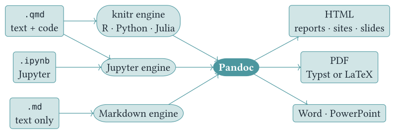
quarto render report.qmd runs your code, then hands Markdown to Pandoc:

Flowchart: a .qmd goes to either the knitr engine or the Jupyter engine, an .ipynb goes to the Jupyter engine, and a .md goes to the Markdown engine. All three engines feed Pandoc, which renders HTML, PDF, and Word or PowerPoint outputs.

Anatomy of a .qmd

Three parts: a YAML header, Markdown prose, and executable code cells.

---
title: "A penguin report"
format: html
---

We measured **`{r} nrow(penguins)`** penguins.

```{r}
#| label: fig-bill
#| fig-cap: "Bill length versus depth"
ggplot(penguins, aes(bill_len, bill_dep, color = species)) +
  geom_point()
```

Cell options use the #| “hash-pipe”: one YAML option per line.

Lab starter checkpoint

The supplied starter (day1-intro/authoring-starter.qmd) already contains this setup cell:

```{r}
#| label: setup
#| message: false
library(dplyr)
library(ggplot2)
library(gt)
library(ggokabeito)   # color-blind-safe (Okabe-Ito) scale
data(penguins)
penguins <- penguins |> filter(!is.na(bill_len), !is.na(bill_dep))
```

Markdown and content: what changes

If Markdown is new to you, see Markdown Basics.

Quarto adds research-writing features: figures and tables with captions, cross-references (@fig-bill, @tbl-summary, @eq-ratio), math, inline code that reports numbers from the data, and callouts.

Figures & cross-references

A labeled code cell becomes a numbered, referenceable figure:

```{r}
#| label: fig-bill
#| fig-cap: "Bill length versus depth, by species."
#| fig-alt: >-
#|   Scatter plot of bill depth against bill
#|   length for three penguin species,
#|   forming clusters.
#| output-location: column
ggplot(penguins, aes(bill_len, bill_dep,
                     color = species)) +
  geom_point(alpha = 0.8) +
  labs(x = "Bill length (mm)",
       y = "Bill depth (mm)")
```
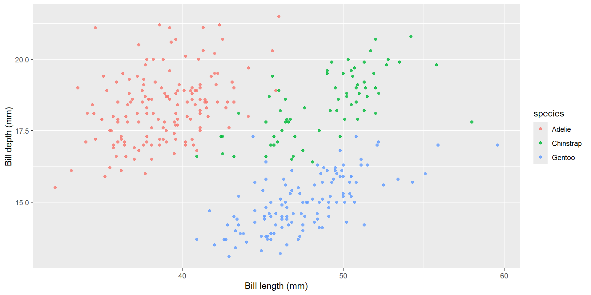
Scatter plot of bill depth against bill length for three penguin species, forming clusters.
Figure 1: Bill length versus depth, by species.

Refer to it in prose with @fig-bill → renders as “Figure 1”, a live link. Labels must start with fig- / tbl- / eq- to be cross-referenceable. #| fig-alt is the figure’s alt text (the description screen readers announce). Add it to every figure.

#| output-location: column is slide-only: a revealjs placement, not article layout.

Tables

gt (or knitr::kable) turns a data frame into a table. A #| label: tbl- makes it referenceable.

```{r}
#| label: tbl-summary
#| tbl-cap: "Mean bill length per species."
penguins |>
  summarise(bill = mean(bill_len), .by = species) |>
  gt() |> fmt_number(bill, decimals = 1)
```
Table 1: Mean bill length per species.
species bill
Adelie 38.8
Gentoo 47.5
Chinstrap 48.8

Then refer to it in prose with @tbl-summary (the same mechanism as figures).

Learn more: Cross-references

Math

Display math with a label is cross-referenceable too:

$$
\text{ratio} = \frac{\text{bill_len}}{\text{bill_dep}}
$$ {#eq-ratio}

This renders as Equation 1 below:

\[ \text{ratio} = \frac{\text{bill_len}}{\text{bill_dep}} \tag{1}\]

Callouts

Callouts are first-class Markdown (no package):

::: {.callout-tip}
Base-R `penguins` (R ≥ 4.5) needs no install.
:::

Tip

Base-R penguins (R ≥ 4.5) needs no install.

::: {.callout-note}
## About the dataset
Base-R `penguins` (R ≥ 4.5) needs no install.
:::

About the dataset

Base-R penguins (R ≥ 4.5) needs no install.

Learn more: Callouts

Inline code

Inline code inserts a computed value into prose. Put it in a sentence:

We measured `{r} nrow(penguins)` penguins.

It renders with the live count: “We measured 342 penguins.”

The number updates when the data changes.

  • Put the engine name in the braces. {python} and {julia} use the same syntax.
  • Keep inline expressions short. Compute complex values in a cell first, then insert one result.
  • Inline code is not evaluated in document metadata such as title, or in cell options such as #| fig-cap.
  • Inline results are escaped as text. In R, wrap a value in I() to preserve its Markdown formatting.

Learn more: Inline code

Layouts: body, margin, and beyond

The article-layout model puts content in the body, the margin, or a zone wider than the body (in the paged formats: HTML, LaTeX, Typst):

  • page-layout: article / full: the overall grid.
  • margin content: figures, tables, captions, .aside, and footnotes.
  • outset / inset: a figure or table that extends beyond the body (outset) or widens toward the page while keeping a margin from the edge (inset).
  • multi-column ::: {.columns} and panels: tabsets and layout-ncol.

Put output in the margin

A cell’s #| column: margin places its output (figure or table, caption and all) in the margin:

```{r}
#| label: counts
#| column: margin
penguins |> count(species, name = "n") |> knitr::kable()
```

Learn more: Article Layout · Margin content

Make it accessible

Accessibility starts with a few practices:

  • Alt text: add #| fig-alt: to every figure. It is what a screen reader announces.
  • Color-blind-safe colors: choose a suitable palette. Okabe-Ito is a common choice for discrete scales in science (scale_color_okabe_ito()). Viridis suits continuous scales. Encode by shape or label too, not color alone.
  • Check contrast: WCAG AA requires a contrast ratio of at least 4.5:1 for normal text. Quarto’s built-in axe runs axe-core on the rendered page:
format:
  html:
    axe:
      output: document    # or `axe: true` to log to the browser console
      standard: wcag21aa  # the level you are checking against

Learn more: HTML Accessibility

One source → many formats

One format: key selects the output. Shared content can render to more than one format:

format:                   # render several at once
  html: default
  typst: default
toc: true                 # shared: applies to both
format:                   # …or set options per format
  html:
    toc: false
  typst:
    toc: true
  • Shared vs. per-format: top-level keys (toc, number-sections, …) apply to every format. The format: map overrides them per output.
  • Conditional content: show or hide a block per format:
::: {.content-visible when-format="html"}
Only in HTML.
:::
  • The layout idioms adapt per format: write once, target many.

Learn more: Multiple formats · Conditional content

Execution: set once, override per cell

Header — defaults for every cell:

execute:
  echo: false
  warning: false

A cell — overrides locally with #|:

```{r}
#| echo: true
summary(penguins$body_mass)
```

The YAML header sets the defaults. A cell’s option in #| wins.

execute options work across languages. For R-specific knitr options, put the equivalent settings under knitr: in the YAML header:

knitr:
  opts_chunk: 
    collapse: true
    comment: "#>" 
    R.options:
      knitr.graphics.auto_pdf: true

Learn more: Execution options · Cell options

Running & editing

Run Quarto from the CLI, in whatever editor you like:

quarto preview report.qmd   # live-reloading preview
quarto render  report.qmd   # one-off render
  • RStudio, Positron, and VS Code all work. The visual editor (WYSIWYM — what you see is what you mean) is built into the RStudio IDE, and comes to Positron and VS Code through the Quarto extension.

Parameterized reports

quarto render also accepts -P name:value. Use it to override a document parameter and produce one report per sample or species from a single source. (Optional bonus in today’s lab.)

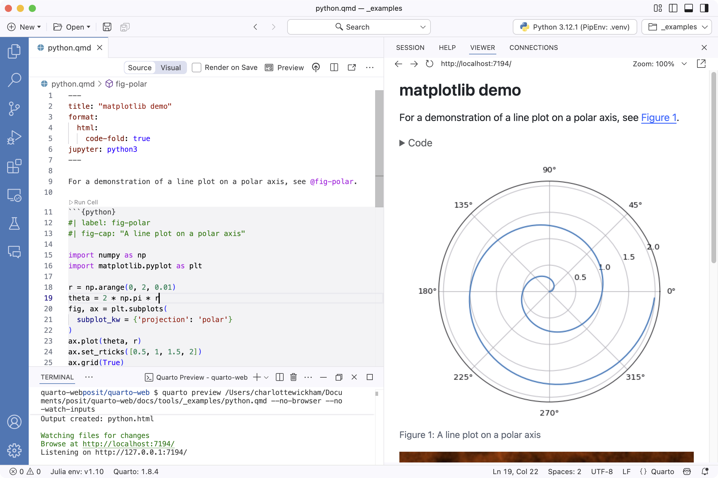
Quarto in Positron

The same quarto preview, from inside the editor: source on the left, live preview on the right. Edit, hit Preview, and it live-reloads.

The Positron IDE with a Quarto document open: a Source/Visual editor toggle and a Preview button above the .qmd source pane on the left, and a live HTML preview of the rendered document on the right.

Your turn

Your turn

Head to the Lab and start at the Authoring Challenge: author a penguins document with a figure, a cross-referenced table, and margin layout, then render it to HTML.

You can now author a figure, a cross-referenced table, and margin layout. After the break we cite it and produce a branded PDF.

Part 2: Citations → Typst

From report to article: cite it, then typeset it.

From report to article

You have a clean HTML document. The lab provides a completed Part-1 report if you need one. To make it a branded article with citations, add two things:

  1. citations: a .bib file and a citation style.
  2. a typeset PDF — via Typst, bundled in Quarto.

Citations

A .bib file holds one entry per source. The entry key is what you cite.

references.bib
@article{gorman2014,
  author = {Gorman, K. B. and ...},
  year   = {2014}
}

Create or export BibTeX entries with Zotero, a DOI lookup, or the journal’s Cite button.

Two header lines point at the file and the style:

bibliography: references.bib
csl: apa.csl

CSL = Citation Style Language. Change csl: to another CSL file to apply that journal’s citation style.

Use brackets to control the citation form:

You write You get
[@gorman2014] (Gorman et al., 2014)
@gorman2014 Gorman et al. (2014)
[-@gorman2014] (2014)

Where the reference list goes

By default the list goes at the end of the document. Put this div where you want it instead:

::: {#refs}
:::

Two processors can build that list, and only one of them reads the div:

  • Pandoc citeproc is the default for HTML. It puts the list in #refs.
  • Typst builds its own bibliography and always places it last.

For the Typst PDF, add citeproc: true so Pandoc processes the citations:

citeproc: true

Learn more: Citations

A real title block

A few header lines add publication metadata (name, affiliation, ORCID, and abstract):

title: "Bill shape distinguishes Antarctic penguins"
author:
  - name: Christophe Dervieux
    affiliation: Posit, PBC
    email: cderv@posit.co
    orcid: 0000-0003-4474-2498
abstract: |
  Using base-R `penguins`, we show bill shape separates species...

The same metadata renders in HTML and a Typst PDF.

Learn more: Authors & Affiliations, Title blocks

Typst — modern PDF, no LaTeX

Typst (https://typst.app/) is a modern typesetting system that is bundled with Quarto: nothing to install, no LaTeX toolchain.

format: typst

That is the only change. Then re-render:

quarto render report.qmd

The header selects the output format.

To get the PDF without touching the header, ask for it on the command line instead: quarto render report.qmd --to typst.

Version check

Typst is bundled from Quarto 1.4+. We require ≥ 1.9 for margin and article layout. Check once with quarto --version.

Branding the PDF — _brand.yml

One _brand.yml carries your palette + fonts to a Typst PDF, and to the plots and tables inside it:

_brand.yml
color:
  palette:
    teal: "#4C979F"
  primary: teal
typography:
  fonts:
    - family: Albert Sans
      source: google
  base:
    family: Albert Sans
  • Same file themes HTML and Typst.
  • The R side (theme_brand_ggplot2() / theme_brand_gt() from the brand.yml package) themes your plots and tables from the same palette.
  • Quarto fetches Google fonts for Typst automatically.

Brand YAML logo: a multicolor circular icon beside the words BRAND YAML.

Learn more: Quarto brand · brand.yml spec

Your turn

Your turn

Return to the Citations Challenge in the Lab. Add citations to my-report.qmd (save authoring-checkpoint.qmd as my-report.qmd if you did not finish Part 1), then render it as a branded Typst PDF.

What you can do now

You can now:

  • author a .qmd natively with figures, tables, cross-references, math, and callouts.
  • lay it out with the article grid and margin content.
  • make it accessible with alt text, color-blind-safe colors, and a built-in axe check.
  • cite it with a .bib and CSL, and give it a real title block.
  • render it as a branded Typst PDF.

Next (Day 2): grow one document into a whole project, a website your team can publish.
Thank you!

Questions?

Christophe Dervieux · GitHub @cderv · cderv@posit.co