Introduction to Quarto — Lab

RaukR 2026 · Day 1

Scope

Build one penguins document with the authoring extras, then cite it and render it as a branded Typst PDF. You will use one document for two challenges, with a break between them. The result follows the same path from an analysis to a submission-ready report. Everything runs on base-R datasets::penguins (R ≥ 4.5), so there is no data to download.

Before you start: work through the Setup page if you haven’t. The 00-check-setup.R script is at the top of the exercises download (not inside day1-intro/). It confirms R, Quarto, and the packages this lab uses.

You are working in the day1-intro/ folder from the exercises download. Open that folder in your editor, or make it your working directory in R (see the Setup page). Everything you render is written next to your files. Start with the supplied authoring-starter.qmd. The lab introduces the other files when you need them. The folder README lists them all.

The folder also holds a _brand.yml. Quarto applies it to anything you render there, so your HTML carries the RaukR font and colors from the first render.

Coming from R Markdown? (optional)

You do not need to convert anything to work natively in Quarto. Start with .qmd directly. But if you have an .Rmd you want to bring over:

it renders as-is (Quarto reads .Rmd too).
cell options move from the chunk header to the #| “hash-pipe” (one YAML option per line).
knitr::convert_chunk_header("doc.Rmd", output = "doc.qmd") does the mechanical part.

The rest of this lab uses native .qmd.

1 Authoring Challenge

Goal: a penguins report with a cross-referenced figure, a cross-referenced table, and a margin element, rendered to HTML.

Starting point. Open day1-intro/authoring-starter.qmd and save it as my-report.qmd, in that same folder (next to references.bib / apa.csl / _brand.yml, so Part 2’s paths resolve later). Render it once to confirm it works, then re-render after every step below.

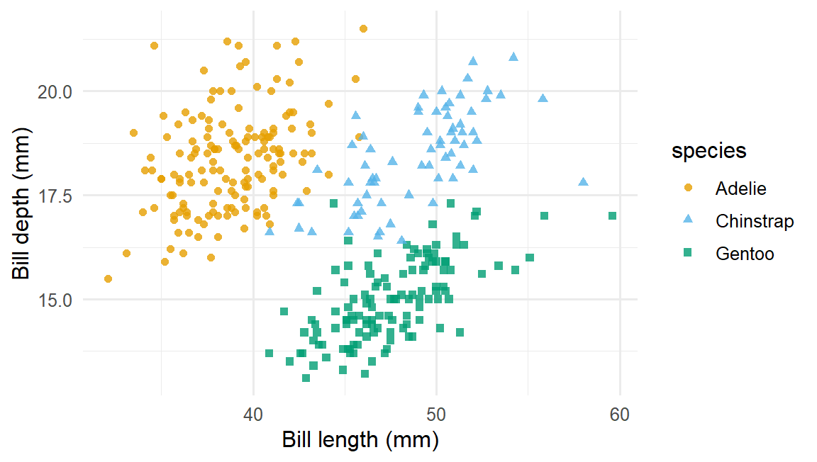
The starter is already a working report, but it has no captions, cross-references, or alt text. Most steps require no R changes. The accessibility step makes three small changes to the plot.

Most steps use cell options. A cross-reference has two ends: a labeled target and an @label in the prose that points at it. For figures and tables, add a cell label with the right prefix (fig- or tbl-) and a caption. (A cell is what R Markdown calls a chunk.) An equation label (eq-) attaches to the closing $$ instead. Layout also uses a cell option. Each step links to the relevant documentation.

Missing the download? Take the source directly:

authoring-starter.qmd

1.1 Cross-reference the figure

Goal. Turn the scatter plot into a numbered figure with a caption, and refer to that number from the prose. Two edits: an option on the cell, and a reference in the body text above it.

Quarto docs

Cross-references

You should see

A caption Figure 1: … under the plot, and a sentence above it containing a live Figure 1 link.

Hint

Which cell options tell Quarto to number this figure, and how do you refer to it in the text?

A cell becomes cross-referenceable when its label starts with a known prefix (fig- for a figure) and is unique in the document. The caption is a second cell option. Label, caption and the @fig-something reference work together: a reference with no matching label renders as ?@fig-something.

Solution

On the plot cell:

#| label: fig-bill
#| fig-cap: "Bill length versus depth, colored by species."

And the sentence above the cell, rewritten to point at it:

@fig-bill shows that within a species the bill has a characteristic shape, so the species form
clusters.

1.2 Cross-reference the table

Goal. Apply the same method to the summary table under Mean measurements: a numbered, captioned Table 1, introduced by a sentence that links to it. The gt call is already written. That section has no prose yet, so add the sentence.

Quarto docs

Cross-references for tables

You should see

Table 1: … above the table (table captions go above, figure captions below), and a sentence introducing it with a live Table 1 link.

Hint

Figures and tables are numbered in separate sequences. Which label prefix tells Quarto this one is a table?

Use #| label: tbl-summary and #| tbl-cap: on the cell, then @tbl-summary in the prose. The prefix decides both the sequence and the word (“Figure”, “Table”) Quarto prints.

Solution

On the gt cell:

#| label: tbl-summary
#| tbl-cap: "Mean measurements per species."

And above it:

@tbl-summary reports the mean bill measurements and body mass per species.

1.3 Move the counts into the margin

Goal. Put the species-counts table in the right margin, beside the paragraph that mentions it, instead of in the main text column. The column: cell option controls this. The linked documentation lists its values.

Quarto docs

Article layout

You should see

The counts table in the right-hand margin, beside the counts cell, and the main text column unchanged in width.

Hint

The R code does not change. Add #| column: margin to the cell. That option also takes body, body-outset, page and screen. For prose rather than cell output, use a ::: {.column-margin} div.

Solution

On the counts cell:

#| column: margin

1.4 Make the figure accessible

Goal. Make the figure readable by someone who cannot distinguish the colors, and by someone using a screen reader.

The plot separates species by color alone, in ggplot2’s default palette, which is not color-blind-safe. This is the one step that edits the R: three changes to the plot, one option on the cell. ggokabeito is already loaded in the setup cell and supplies scale_*_okabe_ito().

Quarto docs

HTML accessibility · Figure alt text

You should see

Each species drawn with its own shape as well as its own color, in the Okabe-Ito palette (orange, blue, green rather than ggplot2’s salmon, green and blue), and one legend for both color and shape. If you get two stacked legends instead, give the shape legend the same title as the color legend. The alt text is not visible on the page: to check it, view the page source and confirm the <img> tag carries your alt="…". The finished figure looks like this:

Scatter plot of bill depth against bill length for three penguin species. Each species uses a distinct color and point shape. The points form three largely separate clusters. — Figure 1: Target: bill length versus depth by species.

Hint

Someone who cannot separate the three colors needs a second way to tell the species apart. What else can aes() map? Where does the plot description go when the other figure settings are cell options?

Map shape = species alongside color = species in aes(), and add scale_color_okabe_ito(). The description is the cell option #| fig-alt:. It is not the caption: alt text conveys the information in the image, so describe what the plot shows rather than merely naming the plot type.

Solution

On the plot cell, next to the label and caption:

#| fig-alt: >-
#|   Scatter plot of bill depth against bill length for penguins of three species, each drawn in a
#|   distinct color and shape. The three species form largely separate clusters.

And in the plot itself:

ggplot(penguins, aes(bill_len, bill_dep, color = species, shape = species)) +
  geom_point(alpha = 0.8) +
  scale_color_okabe_ito() +
  labs(x = "Bill length (mm)", y = "Bill depth (mm)", color = "Species", shape = "Species") +
  theme_minimal(base_size = 12)

Naming both color and shape in labs() merges them into a single legend.

Optional accessibility check

Your figure now has alt text and redundant color/shape encoding. To check the whole page, Quarto can run axe-core in the browser. See HTML Accessibility.

Your header still has format: html on one line. The option belongs under that format, so expand it into a block:

format:
  html:
    axe:
      output: document

Re-render, and a panel appears at the bottom of the page. With nothing to report it reads No axe-core violations found. Otherwise each violation is listed with its impact, and hovering a selector highlights the element it points to.

Remove the axe: option before you publish.

1.5 Add a numbered equation (optional)

Goal. Add the bill-shape ratio (bill length divided by bill depth) as a numbered display equation, and refer to it from the prose.

One caution: inside $$…$$, bill_len can render as a subscript, so escape the underscore as bill\_len.

Quarto docs

Equations

You should see

The formula centered on its own line with (1) at the right margin, and the sentence above it linking to that number.

Hint

Display math is not a cell, so the label cannot be a cell option. Where can you attach it?

The label is an attribute on the closing $$, written {#eq-ratio}. The eq- prefix makes it a numbered equation, and @eq-ratio links to it like @fig- and @tbl-.

Solution

A compact descriptor of bill shape is the length-to-depth ratio (@eq-ratio):

$$
\text{ratio} = \frac{\text{bill\_len}}{\text{bill\_dep}}
$$ {#eq-ratio}

You should see

A numbered Figure 1 (the bill scatter, three separate clusters), a numbered Table 1, and the counts in the right margin. Your figure and table references render as live links, with no ?@ markers anywhere. If you completed the optional step, you also have a numbered Equation 1.

authoring-checkpoint.qmd is this same report with every step above applied. It is already in day1-intro/. Compare your work against it, or, if you did not finish, save a copy of it as my-report.qmd and continue into Part 2 from there. You can also take the source:

authoring-checkpoint.qmd

2 Citations Challenge

Goal: cite the report, then render the same document as a branded Typst PDF.

Starting point

If you finished the Authoring Challenge, continue in my-report.qmd. Otherwise:

Open day1-intro/authoring-checkpoint.qmd (the completed Part-1 report).
Save a copy as my-report.qmd in day1-intro/, next to references.bib, apa.csl, and _brand.yml.
Continue in that copy.

The instructions below use my-report.qmd for both routes.

Missing the download? Take the sources directly:

references.bib apa.csl _brand.yml

Quarto docs

Citations · Typst · Conditional content · Brand

2.1 Add the bibliography and citation style

Point the document header at the shared bibliography and citation style. Add citeproc: true so Quarto processes the citations and places the reference list in the #refs div you add below. Without it, Typst processes the citations and ignores that div:

bibliography: references.bib
csl: apa.csl
citeproc: true

2.2 Cite the two sources

Add [@gorman2014] before the period in the sentence ending “…collected at Palmer Station, Antarctica.” Add [@horst2020] immediately after palmerpenguins in the next sentence. The rest of that sentence describes base R, so keep the citation beside the package name. Do not duplicate either sentence.

2.3 Add the References section

Add a References section where the list should appear:

## References {.unnumbered}

::: {#refs}
:::

2.4 Give it a title block

Give it a real title block so the PDF reads as a paper. Replace your document’s author: line (or add one) with:

author:
  - name: Your Name
    affiliation: Your Lab, Your University

2.5 Render to HTML and check the citations

Render to HTML and confirm that both citations resolve as (Gorman et al., 2014) and (Horst et al., 2020), with a reference list holding both entries.

2.6 Render a branded PDF with Typst

Render a branded PDF with Typst. Keep my-report.qmd in day1-intro/ so Quarto can find the supplied _brand.yml. You may see unknown font family warnings on the first render. See Troubleshooting if the final PDF still uses a serif font. Choose one route:

CLI: keep format: html in the header and run:
```
quarto render my-report.qmd --to typst
```
Editor: change the header to format: typst, then render (RStudio’s Render button, or Quarto: Render Document in Positron and VS Code). The editor renders whatever format: is declared, so while the header still says format: html you get HTML, not a PDF.

The PDF is written next to its source in day1-intro/.

2.7 Keep the Session appendix out of the PDF

Look at the end of the PDF. The Session appendix is printed in full, with the sessionInfo() call and all of its output. <details> is an HTML disclosure widget and Typst has no equivalent, so that block belongs to HTML only. Wrap the whole section (the heading and the <details> block) in a conditional div:

::: {.content-visible when-format="html"}

## Session {.appendix .unnumbered}

<!-- Keep the existing <details> block here. -->

:::

Render to Typst again, then to HTML. On the editor route, set format: back to html for that second render. The appendix is gone from the PDF and unchanged in the HTML.

You should see

In-text (Gorman et al., 2014) and (Horst et al., 2020), a References section formatted in APA with both entries, and the same citations in the Typst PDF, typeset with the RaukR palette. No ?@gorman2014, ?@horst2020 or [?] markers anywhere.

The entries sit inside the ::: {#refs} div in both formats, under your own References heading. The PDF ends there, with no Session appendix after it. The HTML still includes the appendix, with the Session block collapsed.

Check that the branding is applied. An unbranded PDF builds without any error, so check the title and headings. A branded PDF uses Albert Sans. An unbranded PDF uses Typst’s default serif. Table 1 remains serif in both because of the unknown font family issue described in Troubleshooting. Use the headings for this check. Serif headings mean _brand.yml isn’t next to your .qmd.

Hint

The @key in [@gorman2014] must match a key in references.bib exactly.
csl: sets the style (here APA). Swap the file to restyle every citation at once.
content-visible has an inverse, content-hidden. ::: {.content-hidden when-format="typst"} says the same thing the other way round.
The first Typst render requires a network connection while Quarto downloads the brand’s Google fonts.

Solution: the header and citations

In the YAML header:

bibliography: references.bib
csl: apa.csl
citeproc: true

In the prose, append each citation to the sentence that credits its source:

… collected at Palmer Station, Antarctica [@gorman2014]. The data are available through the
**palmerpenguins** package [@horst2020] and are now also included in base R's `datasets` package.

A References section (the list renders inside the #refs div):

## References {.unnumbered}

::: {#refs}
:::

The Session appendix, kept out of the PDF:

::: {.content-visible when-format="html"}

## Session {.appendix .unnumbered}

<!-- Keep the existing <details> block here. -->

:::

For the branded PDF (day1-intro/_brand.yml styles it), either force the target from the CLI:

quarto render my-report.qmd --to typst

or set format: typst in the header and render from the editor.

solutions/day1/penguins-report.qmd is the complete Day-1 report: the starter with every step of both challenges applied. Try the challenge first, then open it to compare, or take the source:

penguins-report.qmd

For a more advanced branded PDF example, render day1-intro/sample-typst.qmd. It also styles its table and plot in R and sets Typst page options. Those additions are outside this exercise.

3 Bonus — one report per species (optional)

Goal: turn a report into a parameterized one: a single source that renders a separate report per species by passing the species at render time. This section is optional. Skip it if time is short.

A parameter is a value declared in the YAML that your code can read as params$…. Change the value at render time and the same document produces a different report. You do not need separate source files.

Starting point

Open day1-intro/parameters-starter.qmd. It contains the report structure, data, and plot. Your task is to make the species an input to the document. A complete reference is available at solutions/day1/penguins-by-species.qmd.

Missing the download? Take the source directly:

parameters-starter.qmd

Tasks

Declare a parameter with a default in the header:
```
params:
  species: Gentoo
```
Use it to filter in the setup cell. params$species is a value. Keep the existing missing-value checks and add the species condition:
```
one <- penguins |> filter(species == params$species, !is.na(bill_len), !is.na(bill_dep))
```
Use the parameter in the report. Three places, marked TODO 3a, 3b and 3c in the file. Replace the placeholder species in the opening sentence with inline code (`{r} params$species`), and name the species in the closing sentence the same way. Make the caption and alt text track the parameter with !expr. Cell options are YAML, so the !expr tag tells Quarto to evaluate the R expression:
```
#| fig-cap: !expr paste0("Bill length versus depth for ", params$species, " penguins.")
#| fig-alt: !expr paste0("Scatter plot of bill depth against bill length for ", params$species, " penguins.")
```
Render a different species from the CLI with -P name:value. Run this from inside day1-intro/:
```
quarto render parameters-starter.qmd -P species:Adelie
```
With no -P, the default (Gentoo) is used.

Quarto docs

Parameters

Optional: dynamic headings and standalone files

Replace Species in the heading with inline code so it shows the selected species:

## `{r} params$species` at a glance

To keep two named reports, render each as a self-contained HTML file:

quarto render parameters-starter.qmd -P species:Adelie    --output adelie.html    --embed-resources
quarto render parameters-starter.qmd -P species:Chinstrap --output chinstrap.html --embed-resources

--output prevents the second render from overwriting the first. --embed-resources puts each plot inside its HTML file, so the reports do not share a figure-support folder.

You should see

Rendering with -P species:Adelie gives a report whose sentences, figure caption, alt text, point count, and plot are all about Adelie. No text or plot data refer to Gentoo. Rendering without -P produces the Gentoo report. If you completed the optional task, the heading also names the selected species.

Hint

Parameters must have defaults: params$species has to resolve when no -P is passed.
-P takes name:value (-P species:Adelie). Pass several with repeated -P flags.
The plot must use the filtered object one, not the full penguins data.

The complete, runnable solution is solutions/day1/penguins-by-species.qmd. Open it to compare your work or render it with different -P species: values. You can also take the source:

penguins-by-species.qmd

4 Troubleshooting

If rendering fails or the output looks wrong

YAML is indentation-sensitive. If rendering fails before any code runs, check the YAML header for stray spaces, tabs, or unmatched quotes.
Missing package? install.packages("<name>") (or renv::restore()) and render again.
A cross-reference shows ?@…? For a figure or table, confirm that the cell label starts with fig- or tbl-. For an equation, confirm that {#eq-…} follows the closing $$. Then make sure the @ref matches the label exactly.
A citation shows ?@gorman2014 or [?]? The @key doesn’t match a key in references.bib, or bibliography: isn’t set.
The PDF’s References section is empty and the entries are at the end under “Bibliography”? citeproc: true is missing from the header. Without it Typst builds the bibliography itself and places it last, so the ::: {#refs} div only moves the list in HTML.
references.bib not found, although the download has it? Your .qmd is probably not in day1-intro/ (saved to the top folder, for example). Move it next to references.bib / apa.csl / _brand.yml and render again.
Do I need to install Typst? No. Typst is bundled in Quarto ≥ 1.9, so there’s nothing extra to install (no LaTeX either). Check quarto --version.
Typst PDF looks unbranded / wrong fonts? An unbranded render can succeed without a warning, so check the title and headings, not the log. A branded PDF uses Albert Sans. An unbranded PDF uses Typst’s default serif. Table 1 stays serif either way, so don’t judge by the table. Confirm _brand.yml is in your day1-intro/ folder (next to the .qmd) and you have network on the first render (Quarto fetches the Google fonts once). Missing the file? Download _brand.yml into the folder holding your .qmd.
Typst prints unknown font family warnings? A gt table names a generic sans-serif in its font stack, and Typst doesn’t recognize that as a family. The warning does not stop the PDF from building or applying the brand.

Session

Session info

sessionInfo()

R version 4.6.1 (2026-06-24 ucrt)
Platform: x86_64-w64-mingw32/x64
Running under: Windows 11 x64 (build 26200)

Matrix products: default
  LAPACK version 3.12.1

locale:
[1] C
system code page: 65001

time zone: Europe/Paris
tzcode source: internal

attached base packages:
[1] stats     graphics  grDevices datasets  utils     methods   base     

other attached packages:
[1] ggokabeito_0.1.0 gt_1.3.0         ggplot2_4.0.3    dplyr_1.2.1     

loaded via a namespace (and not attached):
 [1] vctrs_0.7.3        cli_3.6.6          knitr_1.51         rlang_1.3.0       
 [5] xfun_0.59          renv_1.2.3         generics_0.1.4     S7_0.2.2          
 [9] jsonlite_2.0.0     labeling_0.4.3     glue_1.8.1         htmltools_0.5.9   
[13] scales_1.4.0       rmarkdown_2.31     grid_4.6.1         evaluate_1.0.5    
[17] tibble_3.3.1       fastmap_1.2.0      yaml_2.3.12        lifecycle_1.0.5   
[21] compiler_4.6.1     fs_2.1.0           RColorBrewer_1.1-3 htmlwidgets_1.6.4 
[25] pkgconfig_2.0.3    farver_2.1.2       digest_0.6.39      R6_2.6.1          
[29] tidyselect_1.2.1   pillar_1.11.1      magrittr_2.0.5     withr_3.0.3       
[33] tools_4.6.1        gtable_0.3.6       xml2_1.6.0